Cell Bender Functionality & Plotting
Compiled: May 11, 2026
Source:vignettes/articles/Cell_Bender_Functions.Rmd
Cell_Bender_Functions.RmdCellBender Functionality
CellBender is software for elimination of technical artifacts in scRNA-seq/snRNA-seq that uses deep generative model for unsupervised removal of ambient RNA and chimeric PCR artifacts. You can find out more info about CellBender from the bioRxiv Preprint, GitHub Repo, and Documentation.
Following completion of CellBender scCustomize contains a couple of functions that may be helpful when creating and visualizing data in Seurat.
library(ggplot2)
library(dplyr)
library(magrittr)
library(patchwork)
library(viridis)
library(Seurat)
library(scCustomize)
library(qs2)
Importing Cell Bender H5 Outputs
The output from CellBender is an H5 file that is styled and can be
read like 10X Genomics H5 file. In CellBender pre-v3 this file could be
read by Seurat::Read10X_h5() (although that function
assumes that the file contains no name prefix). However, v3+ contains
extra information that causes Read10X_h5 to fail.
scCustomize contains function Read_CellBender_h5_Mat()
can be used when reading in CellBender h5 files regardless of the
version of CellBender used.
cell_bender_mat <- Read_CellBender_h5_Mat(file_name = "PATH/SampleA_out_filtered.h5")Importing CellBender data based on STARsolo or pre-V3 Cell Ranger inputs
If the input that CellBender uses is based on STARsolo or pre-V3 Cell
Ranger data then some of the slot name which stores feature/gene ids in
the H5 file is different. These files can be read by specifying the
optional feature_slot_name parameter.
cell_bender_starsolo_mat <- Read_CellBender_h5_Mat(file_name = "PATH/SampleA_out_filtered.h5", feature_slot_name = "genes")Importing CellBender data with non-standard group names
If CellBender H5 file contains non-standard H5 group names then
Read_CellBender_h5_Mat will error. To circumvent this
simply supply the name of the H5 group that contains the count data.
cell_bender_name_mat <- Read_CellBender_h5_Mat(file_name = "PATH/SampleA_out_filtered.h5", h5_group_name = "background_removed")Reading multiple CellBender files with single function
scCustomize also contains two wrapper functions to easily read
multiple CellBender files stored either in single directory or in
multiple sub-directories Read_CellBender_h5_Multi_File and
Read_CellBender_h5_Multi_Directory.
Read in H5 outputs from multiple sub-directories with
Read_CellBender_h5_Multi_Directory().
Cell Bender Output Structure
The following is typical output directory structure for Cell Bender files with sub-directory labeled with sample name and each file also prefixed with the sample name.
Parent_Directory
├── sample_01
│   └── sample_01_out_cell_barcodes.csv
│   └── sample_01_out_filtered.h5
│   └── sample_01_out.h5
│   └── sample_01_out.log
│   └── sample_01_out.pdf
└── sample_02
│   └── sample_02_out_cell_barcodes.csv
│   └── sample_02_out_filtered.h5
│   └── sample_02_out.h5
│   └── sample_02_out.log
│   └── sample_02_out.pdf
Read Files
All we have to do is adjust the parameters to account for cell bender file names and directory structure.
-
secondary_pathIn this case we can leave asNULLbecause samples are located in immediate subdirectory (secondary path must be the same for all samples). -
custom_name = "_out.h5"This specifies what the common file suffix of all files are.
Optional Parameters
* parallel and num_cores to use multiple core
processing. * sample_list By default
Read_CellBender_h5_Multi_Directory will read in all
sub-directories present in parent directory. However a subset can be
specified by passing a vector of sample directory names. *
sample_names As with other functions by default
Read_CellBender_h5_Multi_Directory will use the
sub-directory names within parent directory to name the output list
entries. Alternate names for the list entries can be provided here if
desired. These names will also be used to add cell prefixes if
merge = TRUE (see below).
* merge logical (default FALSE). Whether to combine all
samples into single sparse matrix and using sample_names to
provide sample prefixes.
cell_bender_merged <- Read_CellBender_h5_Multi_Directory(base_path = "assets/Cell_Bender_Example/",
    custom_name = "_out.h5", sample_names = c("WT1", "WT2"), merge = TRUE)
Read in H5 outputs from single directory with
Read_CellBender_h5_Multi_File().
If all output files are in single directory you can use
Read_CellBender_h5_Multi_File to read in all of the files
with single function.
Parent_Directory
├── CellBender_Outputs
│   └── sample_01_out.h5
│   └── sample_02_out.h5
cell_bender_merged <- Read_CellBender_h5_Multi_File(data_dir = "assets/Cell_Bender_Example/", custom_name = "_out.h5",
    sample_names = c("WT1", "WT2"))
Create Seurat Object with Corrected Counts
Creating a Seurat object from merged CellBender matrices then is identical to creating any other Seurat object.
cell_bender_seurat <- CreateSeuratObject(counts = cell_bender_merged, names.field = 1, names.delim = "_")Creating Dual Assay Objects
Sometimes it can be helpful to create object that contains both the
cell ranger values and cell bender values (we’ll come to why below).
scCustomize contains a helper function
Create_CellBender_Merged_Seurat() to handle object creation
in one quick step.
For this function we assume that we will use the cell calling algorithm of Cell Ranger with the modified counts for Cell Bender.
Read in both sets of data
cell_bender_merged <- Read_CellBender_h5_Multi_Directory(base_path = "assets/Cell_Bender_Cell_Ranger_Data/Cell_Bender_Example/",
    custom_name = "_out.h5", sample_names = c("WT1", "WT2"), merge = TRUE)

cell_ranger_merged <- Read10X_h5_Multi_Directory(base_path = "assets/Cell_Bender_Cell_Ranger_Data/Cell_Ranger_Example/",
    default_10X_path = FALSE, h5_filename = "filtered_feature_bc_matrix.h5", merge = TRUE, sample_names = c("WT1",
        "WT2"), parallel = TRUE, num_cores = 2)
Create Dual Assay Seurat Object
To run the function the user simply needs to provide the names of the two matrices and a name for assay containing the Cell Ranger counts (by default this is named “RAW”).
dual_seurat <- Create_CellBender_Merged_Seurat(raw_cell_bender_matrix = cell_bender_merged, raw_counts_matrix = cell_ranger_merged,
    raw_assay_name = "RAW")
Optional Parameters
Users can specify any additional parameters normally passed to
Seurat::CreateSeuratObject() when using this function.
dual_seurat <- Create_CellBender_Merged_Seurat(raw_cell_bender_matrix = cell_bender_merged, raw_counts_matrix = cell_ranger_merged,
    raw_assay_name = "RAW", min_cells = 5, min_features = 200)
Pre/Post Cell Bender Analysis
It can be very important with tools like Cell Bender to analyze how much the process has effected data on a per cell basis.
Add Pre/Post to Meta Data
scCustomize includes function Add_CellBender_Diff() to
help with this process. This function will take the nCount and nFeature
statistics from both assays in the object and calculate the difference
and return 2 new columns (“nCount_Diff” and “nFeature_Diff”) to the
object meta.data.
dual_seurat <- Add_CellBender_Diff(seurat_object = dual_seurat, raw_assay_name = "RAW", cell_bender_assay_name = "RNA")

head(dual_seurat@meta.data, 5)| orig.ident | nCount_RNA | nFeature_RNA | nCount_RAW | nFeature_RAW | nFeature_Diff | nCount_Diff | |
|---|---|---|---|---|---|---|---|
| WT1_AAACCCAAGCGACCCT-1 | WT1 | 9844 | 3423 | 10032 | 3481 | 58 | 188 |
| WT1_AAACCCAAGGAGGCAG-1 | WT1 | 9248 | 3477 | 9431 | 3531 | 54 | 183 |
| WT1_AAACCCACACACCAGC-1 | WT1 | 3207 | 1699 | 3472 | 1852 | 153 | 265 |
| WT1_AAACCCACATCTGTTT-1 | WT1 | 14328 | 3930 | 14572 | 3993 | 63 | 244 |
| WT1_AAACCCAGTATTCTCT-1 | WT1 | 12034 | 3911 | 12223 | 3958 | 47 | 189 |
Calculate per sample averages
We can then use Median_Stats() to calculate per sample
averages across all cells by supplying the new variables to the
median_var parameter.
median_stats <- Median_Stats(seurat_object = dual_seurat, group.by = "orig.ident", median_var = c("nCount_Diff",
"nFeature_Diff"))| orig.ident | Median_nCount_RNA | Median_nFeature_RNA | Median_nCount_Diff | Median_nFeature_Diff |
|---|---|---|---|---|
| WT1 | 7724.5 | 2936 | 216 | 73 |
| WT2 | 7404.5 | 2803 | 212 | 61 |
| Totals (All Cells) | 7565.0 | 2869 | 214 | 67 |
Examine most changed features
It can also be helpful to understand what features may have changed
the most. scCustomize provides the function
CellBender_Feature_Diff to determine changes in features.
This will return a data.frame with rowSums for each feature, the
difference in each feature, and the percent change of each feature.
feature_diff <- CellBender_Feature_Diff(seurat_object = dual_seurat, raw_assay = "RAW", cell_bender_assay = "RNA")| Raw_Counts | CellBender_Counts | Count_Diff | Pct_Diff | |
|---|---|---|---|---|
| Gm42418 | 256834 | 3198 | 253636 | 98.75484 |
| Uqcr11 | 1315 | 20 | 1295 | 98.47909 |
| Gm48099 | 277 | 5 | 272 | 98.19495 |
| Tmsb4x | 6010 | 116 | 5894 | 98.06988 |
| Rps21 | 2597 | 61 | 2536 | 97.65114 |
Plot feature differences
In addition to returning the data.frame it can be useful to visually
examine the changes/trends after running CellBender. The function
CellBender_Diff_Plot takes the data.frame from
CellBender_Feature_Diff as input and plots the results.
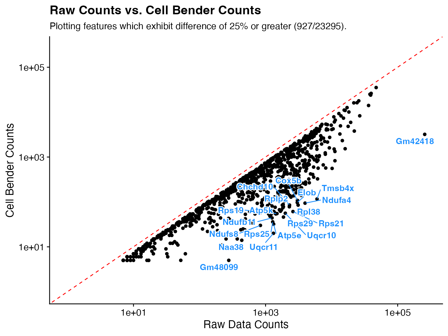
Optional Parameters
-
pct_diff_thresholdplot genes that exhibit a change equal to or greater than this threshold.
-
num_featuresinstead of plotting genes above a threshold simply plot the top X changed genes.
-
num_labelschange how many genes are labeled.
-
labellogical, whether or not to label features.
-
custom_labelsspecify vector of specific features to label.
p1 <- CellBender_Diff_Plot(feature_diff_df = feature_diff)
p2 <- CellBender_Diff_Plot(feature_diff_df = feature_diff, pct_diff_threshold = 50)
p3 <- CellBender_Diff_Plot(feature_diff_df = feature_diff, num_features = 500, pct_diff_threshold = NULL)
p4 <- CellBender_Diff_Plot(feature_diff_df = feature_diff, num_labels = 10)
p5 <- CellBender_Diff_Plot(feature_diff_df = feature_diff, label = F)
p6 <- CellBender_Diff_Plot(feature_diff_df = feature_diff, custom_labels = "Gm48099")

wrap_plots(p1, p2, p3, p4, p5, p6, ncol = 2)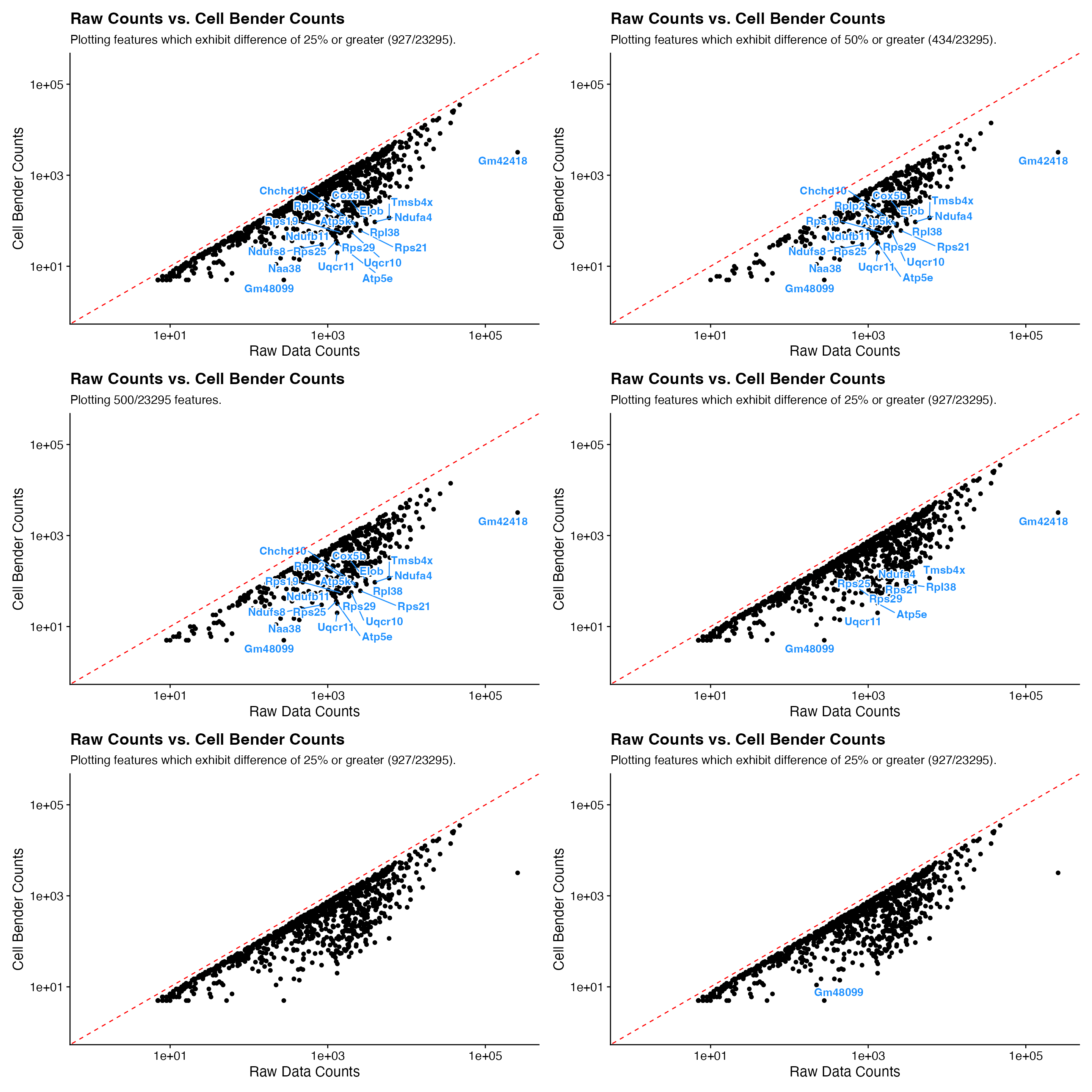
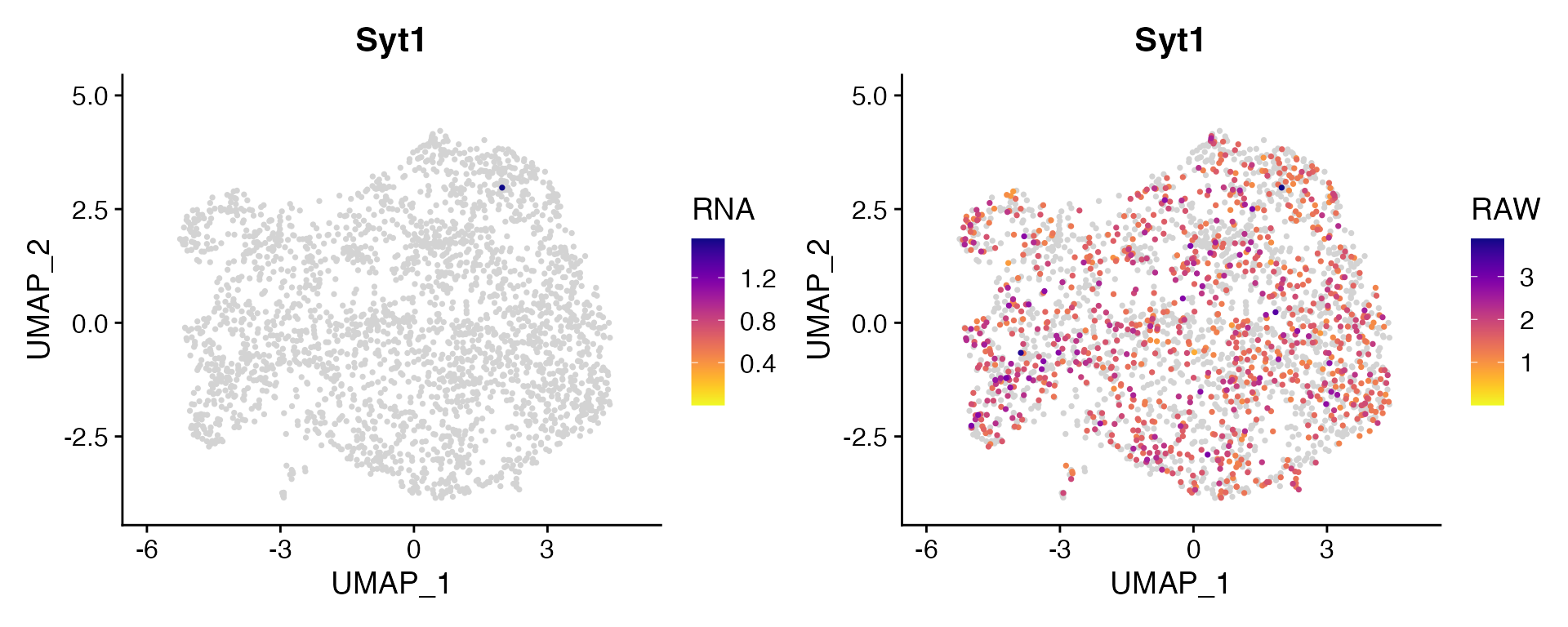
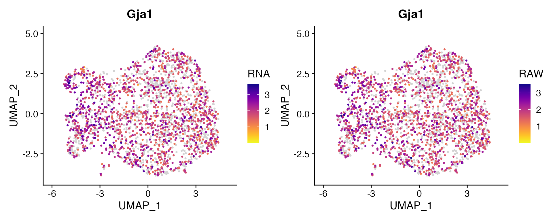
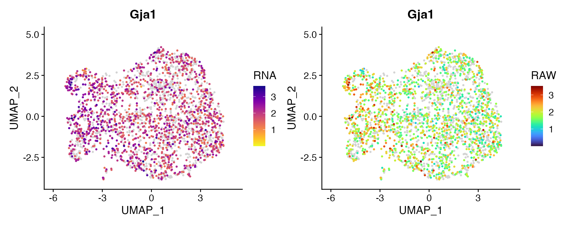
Dual Assay Plotting
For Cell Bender especially, but also potentially for other assays as
well, it can be helpful during analysis to plot the corrected and
uncorrected counts for given feature. scCustomize contains function
FeaturePlot_DualAssay() to make easy.
Users just need to supply the names of the two assays to plot and the features. NOTE: Make sure both assays have been normalized before plotting. The function will attempt to check and make sure both assays have been normalized but has not been tested in all scenarios.
Example Plotting
For this example I’m using unpublished single nucleus RNA dataset from mouse cortex and have subsetted the astrocytes.