Statistics Functions
Compiled: May 11, 2026
Source:vignettes/articles/Statistics.Rmd
Statistics.RmdStatistics Functions
scCustomize contains a couple simple helper functions to return metrics of interest.
For this vignette I will be utilizing pbmc3k dataset from the SeuratData package.
# Load Packages
library(ggplot2)
library(patchwork)
library(dplyr)
library(magrittr)
library(Seurat)
library(scCustomize)

# Load example dataset for tutorial
pbmc <- pbmc3k.SeuratData::pbmc3k.final
Now let’s add some extra meta data for use with tutorial
# Add mito and ribo data
pbmc <- Add_Mito_Ribo(object = pbmc, species = "human")

# Add random sample and group variables
pbmc$orig.ident <- sample(c("sample1", "sample2", "sample3", "sample4"), size = ncol(pbmc), replace = TRUE)
pbmc@meta.data$group[pbmc@meta.data$orig.ident == "sample1" | pbmc@meta.data$orig.ident == "sample3"] <- "Group 1"
pbmc@meta.data$group[pbmc@meta.data$orig.ident == "sample2" | pbmc@meta.data$orig.ident == "sample4"] <- "Group 2"


pbmc@meta.data$treatment[pbmc@meta.data$orig.ident == "sample1"] <- "Control"
pbmc@meta.data$treatment[pbmc@meta.data$orig.ident == "sample2" | pbmc@meta.data$orig.ident == "sample4" |
    pbmc@meta.data$orig.ident == "sample3"] <- "Treated"

# Add dummy module score
pbmc <- AddModuleScore(object = pbmc, features = list(c("CD3E", "CD4", "THY1", "TCRA")), name = "module_score")
Cells Per Identity
It can be really helpful to know the number and percentage of cells
per identity/cluster during analysis.
scCustomize provides the Cluster_Stats_All_Samples function
to make this easy.
cluster_stats <- Cluster_Stats_All_Samples(seurat_object = pbmc)

cluster_stats| Cluster | Number | Freq | sample1 | sample2 | sample3 | sample4 | sample1_% | sample2_% | sample3_% | sample4_% |
|---|---|---|---|---|---|---|---|---|---|---|
| Naive CD4 T | 697 | 26.4215315 | 182 | 176 | 179 | 160 | 26.9629630 | 26.3079223 | 27.2036474 | 25.1572327 |
| Memory CD4 T | 483 | 18.3093252 | 141 | 127 | 112 | 103 | 20.8888889 | 18.9835575 | 17.0212766 | 16.1949686 |
| CD14+ Mono | 480 | 18.1956027 | 118 | 126 | 117 | 119 | 17.4814815 | 18.8340807 | 17.7811550 | 18.7106918 |
| B | 344 | 13.0401820 | 79 | 90 | 78 | 97 | 11.7037037 | 13.4529148 | 11.8541033 | 15.2515723 |
| CD8 T | 271 | 10.2729340 | 60 | 65 | 78 | 68 | 8.8888889 | 9.7159940 | 11.8541033 | 10.6918239 |
| FCGR3A+ Mono | 162 | 6.1410159 | 42 | 34 | 40 | 46 | 6.2222222 | 5.0822123 | 6.0790274 | 7.2327044 |
| NK | 155 | 5.8756634 | 43 | 37 | 41 | 34 | 6.3703704 | 5.5306428 | 6.2310030 | 5.3459119 |
| DC | 32 | 1.2130402 | 7 | 10 | 9 | 6 | 1.0370370 | 1.4947683 | 1.3677812 | 0.9433962 |
| Platelet | 14 | 0.5307051 | 3 | 4 | 4 | 3 | 0.4444444 | 0.5979073 | 0.6079027 | 0.4716981 |
| Total | 2638 | 100.0000000 | 675 | 669 | 658 | 636 | 100.0000000 | 100.0000000 | 100.0000000 | 100.0000000 |
By default Cluster_Stats_All_Samples uses “orig.ident”
as the group variable but user can specify any @meta.data
slot variable.
cluster_stats <- Cluster_Stats_All_Samples(seurat_object = pbmc, group.by = "group")

cluster_stats| Cluster | Number | Freq | Group 1 | Group 2 | Group 1_% | Group 2_% |
|---|---|---|---|---|---|---|
| Naive CD4 T | 697 | 26.4215315 | 361 | 336 | 27.0817704 | 25.7471264 |
| Memory CD4 T | 483 | 18.3093252 | 253 | 230 | 18.9797449 | 17.6245211 |
| CD14+ Mono | 480 | 18.1956027 | 235 | 245 | 17.6294074 | 18.7739464 |
| B | 344 | 13.0401820 | 157 | 187 | 11.7779445 | 14.3295019 |
| CD8 T | 271 | 10.2729340 | 138 | 133 | 10.3525881 | 10.1915709 |
| FCGR3A+ Mono | 162 | 6.1410159 | 82 | 80 | 6.1515379 | 6.1302682 |
| NK | 155 | 5.8756634 | 84 | 71 | 6.3015754 | 5.4406130 |
| DC | 32 | 1.2130402 | 16 | 16 | 1.2003001 | 1.2260536 |
| Platelet | 14 | 0.5307051 | 7 | 7 | 0.5251313 | 0.5363985 |
| Total | 2638 | 100.0000000 | 1333 | 1305 | 100.0000000 | 100.0000000 |
Plotting Cluster/Identity Proportions
Understanding the proportion of cells per cluster and how that may
change across a group can be important aspect of single cell analysis.
scCustomize contains function Proportion_Plot to provide
some visualization of cell proportions.
Plotting proportionality can be tricky especially when dealing with
clusters of very disparate sizes (especially small clusters) so plese be
aware to examine raw data as well (see
Cluster_Stats_All_Samples()).
Also note that when splitting plot by group there are now error bars on these plots for interpretation of variance and other plotting methods should be used to convery such information.
Basic Proportion Plots
Proportion_Plot can either return a bar graph or pie
graph depending on parameter value for
Proportion_Plot(seurat_object = pbmc, plot_type = "bar")

Proportion_Plot(seurat_object = pbmc, plot_type = "pie")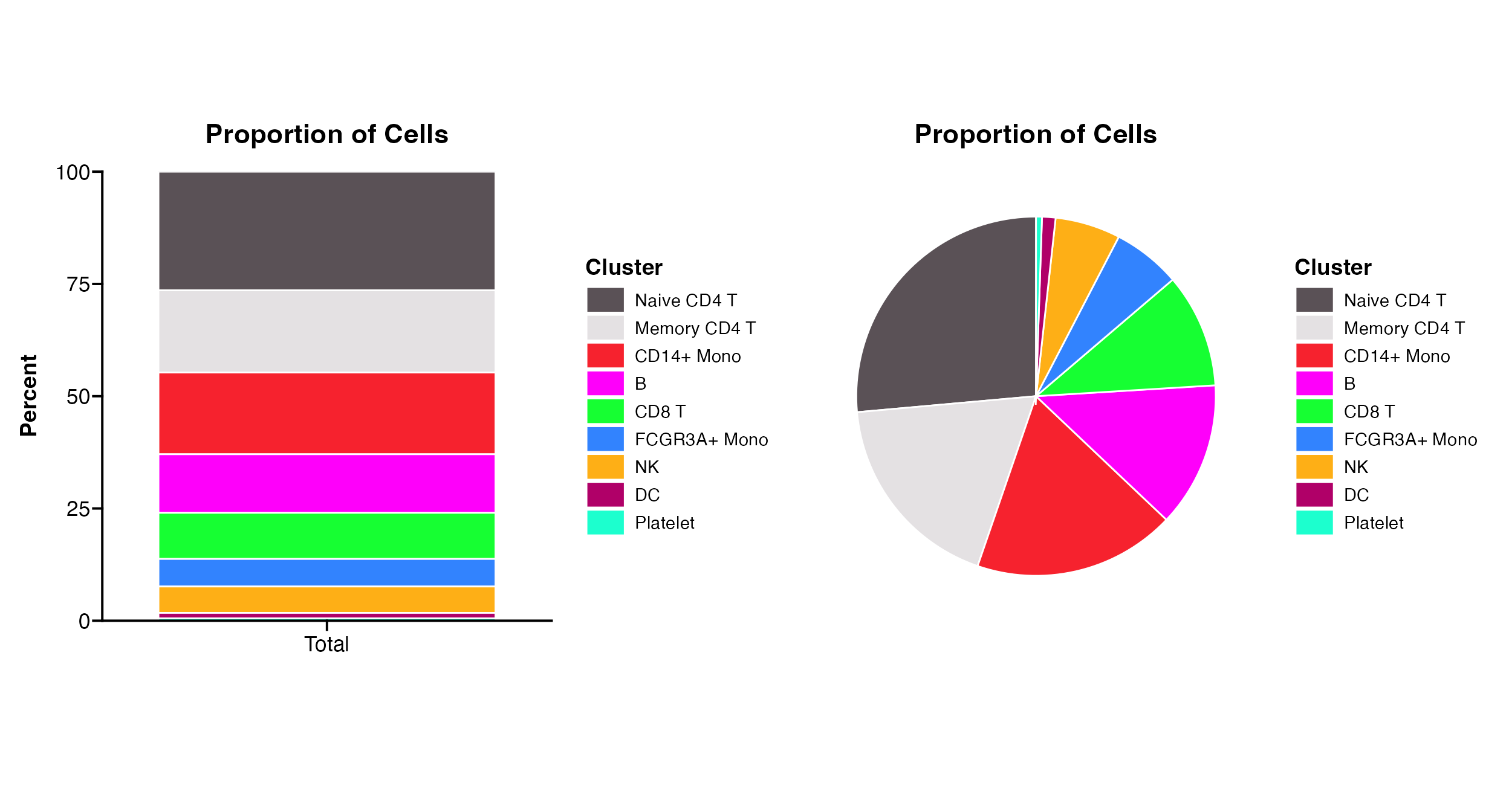
Plot across groups
Like other plots you can also use Proportion_Plot to
split plot across any categorical meta.data variable.
Proportion_Plot(seurat_object = pbmc, plot_type = "bar", split.by = "treatment")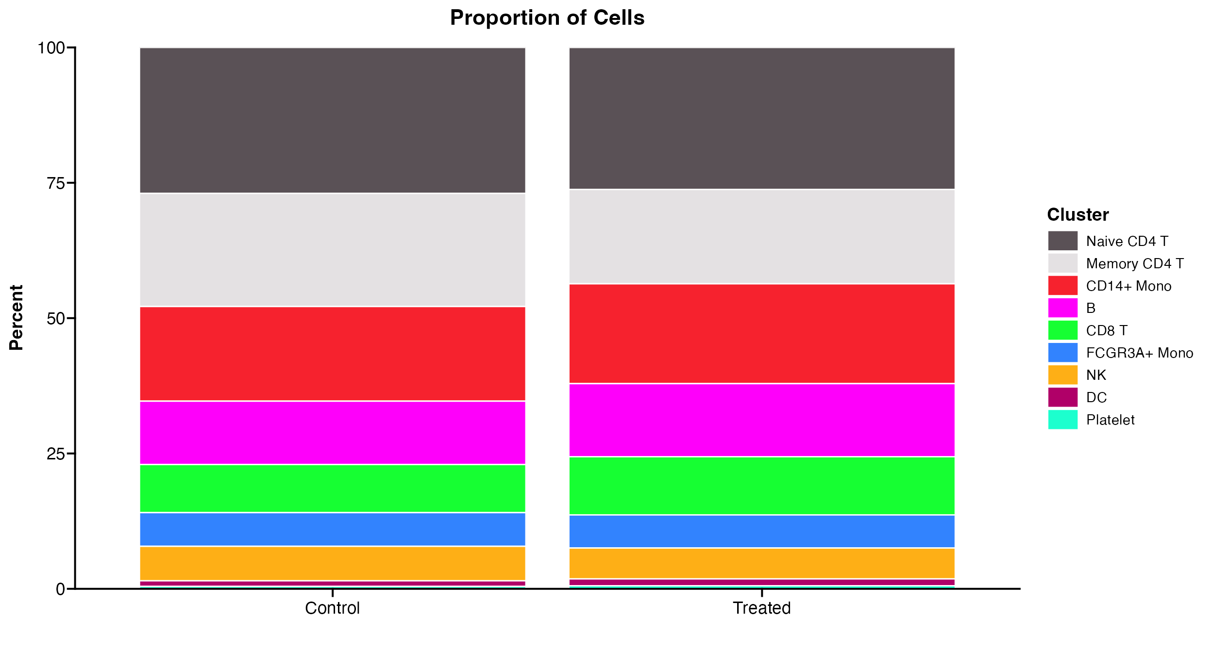
Proportion_Plot(seurat_object = pbmc, plot_type = "pie", split.by = "treatment")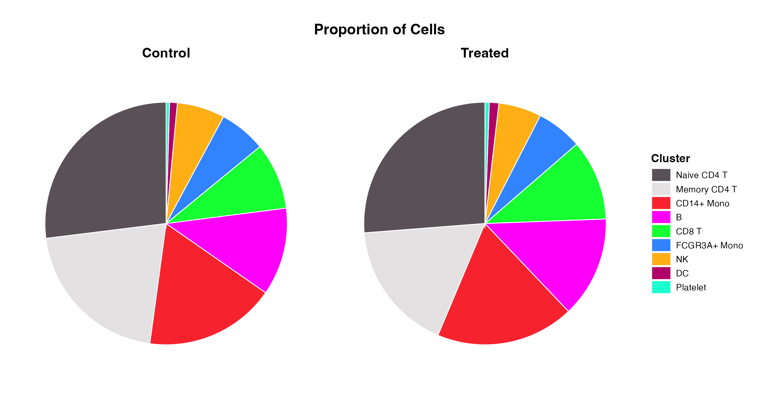
Plot raw cell numbers
The default for Proportion_Plot is to plot the
proportion of cells and not the raw number of cells per identity because
that can be deceptive. However, in some cases it can be useful and so
users can change the plot_scale parameter to plot raw
numbers of cells instead of proportions.
Proportion_Plot(seurat_object = pbmc, plot_type = "bar", split.by = "treatment", plot_scale = "count")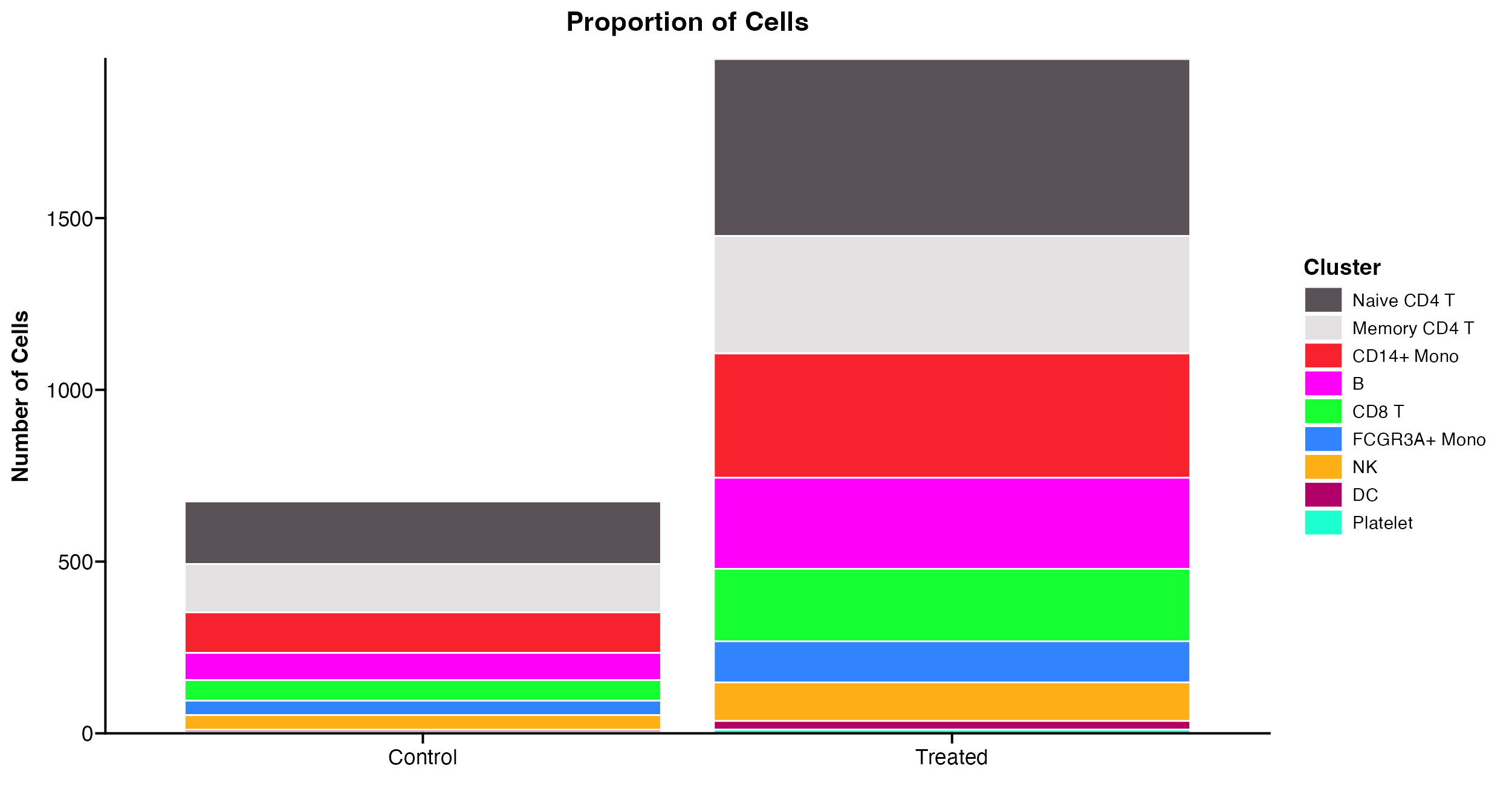
Percent of Cells Expressing Feature(s)
It can also be informative to understand the percent of cells/nuclei
that express a given feature or set of features.
scCustomize provides the Percent_Expressing function to
return these results.
percent_express <- Percent_Expressing(seurat_object = pbmc, features = c("CD4", "CD8A"))| Naive.CD4.T | Memory.CD4.T | CD14..Mono | B | CD8.T | FCGR3A..Mono | NK | DC | Platelet | |
|---|---|---|---|---|---|---|---|---|---|
| CD4 | 6.743185 | 15.942029 | 24.375 | 1.453488 | 2.583026 | 27.160494 | 0.6451613 | 34.375 | 0 |
| CD8A | 13.342898 | 8.902691 | 1.875 | 2.616279 | 50.553505 | 3.703704 | 8.3870968 | 3.125 | 0 |
Change grouping variable
By default the function groups expression across
@active.ident (see above) but user can specify difference
variable if desired.
percent_express <- Percent_Expressing(seurat_object = pbmc, features = c("CD4", "CD8A"), group.by = "orig.ident")| sample3 | sample1 | sample4 | sample2 | |
|---|---|---|---|---|
| CD4 | 11.39818 | 11.55556 | 11.79245 | 12.10762 |
| CD8A | 12.91793 | 12.74074 | 11.00629 | 10.46338 |
Split within groups
User can also supply a split.by variable to quantify
expression within group split by meta data variable
percent_express <- Percent_Expressing(seurat_object = pbmc, features = c("CD4", "CD8A"), split.by = "group")| Naive.CD4.T_Group.1 | Naive.CD4.T_Group.2 | Memory.CD4.T_Group.1 | Memory.CD4.T_Group.2 | CD14..Mono_Group.1 | CD14..Mono_Group.2 | B_Group.1 | B_Group.2 | CD8.T_Group.1 | CD8.T_Group.2 | FCGR3A..Mono_Group.2 | FCGR3A..Mono_Group.1 | NK_Group.1 | NK_Group.2 | DC_Group.2 | DC_Group.1 | Platelet_Group.1 | Platelet_Group.2 | |
|---|---|---|---|---|---|---|---|---|---|---|---|---|---|---|---|---|---|---|
| CD4 | 6.371191 | 7.142857 | 17.39130 | 14.347826 | 24.255319 | 24.48980 | 0.000000 | 2.673797 | 3.623188 | 1.503759 | 31.25 | 23.170732 | 0.000000 | 1.408451 | 37.5 | 31.25 | 0 | 0 |
| CD8A | 13.573407 | 13.095238 | 10.67194 | 6.956522 | 2.553192 | 1.22449 | 1.273885 | 3.743316 | 55.797101 | 45.112782 | 3.75 | 3.658537 | 7.142857 | 9.859155 | 0.0 | 6.25 | 0 | 0 |
Set threshold of expression
Users can also supply a threshold value to quantify percent of cells
expressing feature(s) above a certain threshold (be sure to note which
slot is being used to quantify expression when setting
thresholds).
NOTE: Percent_Expressing currently only supports single
threshold across all features
percent_express <- Percent_Expressing(seurat_object = pbmc, features = c("CD4", "CD8A"), threshold = 2)| Naive.CD4.T | Memory.CD4.T | CD14..Mono | B | CD8.T | FCGR3A..Mono | NK | DC | Platelet | |
|---|---|---|---|---|---|---|---|---|---|
| CD4 | 1.147776 | 0.621118 | 5.8333333 | 0.5813953 | 0.3690037 | 1.851852 | 0.000000 | 3.125 | 0 |
| CD8A | 6.456241 | 2.070393 | 0.2083333 | 0.8720930 | 24.7232472 | 0.000000 | 3.225807 | 0.000 | 0 |
Calculate Summary Median Values
scCustomize contains function Median_Stats to quickly
calculate the medians for basic QC stats (Genes/, UMIs/, %
Mito/Cell).
Basic Use
By default Median_Stats will calculate medians for the
following meta data columns (if present): “nCount_RNA”, “nFeature_RNA”,
“percent_mito”, “percent_ribo”, “percent_mito_ribo”.
median_stats <- Median_Stats(seurat_object = pbmc, group.by = "orig.ident")| orig.ident | Median_nCount_RNA | Median_nFeature_RNA | Median_percent_mito | Median_percent_ribo | Median_percent_mito_ribo |
|---|---|---|---|---|---|
| sample1 | 2193 | 813.0 | 2.005731 | 36.91964 | 39.08969 |
| sample2 | 2178 | 812.0 | 2.016383 | 37.03217 | 39.31227 |
| sample3 | 2241 | 820.0 | 1.982099 | 37.40017 | 39.24930 |
| sample4 | 2251 | 836.5 | 2.057405 | 36.16109 | 38.38636 |
| Totals (All Cells) | 2213 | 819.0 | 2.010702 | 36.92524 | 39.03276 |
Additional Variables
In addition to default variables, users can supply their own
additional meta data columns to calculate medians using the
median_var parameter.
NOTE: The meta data column must be in numeric format (e.g., integer,
numeric, dbl)
median_stats <- Median_Stats(seurat_object = pbmc, group.by = "orig.ident", median_var = "module_score1")| orig.ident | Median_nCount_RNA | Median_nFeature_RNA | Median_percent_mito | Median_percent_ribo | Median_percent_mito_ribo | Median_module_score1 |
|---|---|---|---|---|---|---|
| sample1 | 2193 | 813.0 | 2.005731 | 36.91964 | 39.08969 | -0.0545099 |
| sample2 | 2178 | 812.0 | 2.016383 | 37.03217 | 39.31227 | -0.0678532 |
| sample3 | 2241 | 820.0 | 1.982099 | 37.40017 | 39.24930 | -0.0793297 |
| sample4 | 2251 | 836.5 | 2.057405 | 36.16109 | 38.38636 | -0.1935054 |
| Totals (All Cells) | 2213 | 819.0 | 2.010702 | 36.92524 | 39.03276 | -0.0922378 |
Calculate Median Absolute Deviations
In addition to calculating the median values scCustomize includes
function to calculate the median absolute deviation for each of those
features with function MAD_Stats. By setting the parameter
mad_num the function will retrun the MAD*mad_num.
mad <- MAD_Stats(seurat_object = pbmc, group.by = "orig.ident", mad_num = 2)| orig.ident | MAD x 2 nCount_RNA | MAD x 2 nFeature_RNA | MAD x 2 percent_mito | MAD x 2 percent_ribo | MAD x 2 percent_mito_ribo |
|---|---|---|---|---|---|
| sample1 | 1464.809 | 397.3368 | 1.640639 | 23.92318 | 23.93974 |
| sample2 | 1319.514 | 361.7544 | 1.579981 | 23.47474 | 23.15831 |
| sample3 | 1500.391 | 392.8890 | 1.557364 | 23.57180 | 23.52481 |
| sample4 | 1478.152 | 381.0282 | 1.451580 | 24.44613 | 24.08378 |
| Totals (All Cells) | 1442.570 | 379.5456 | 1.544386 | 23.73656 | 23.38683 |
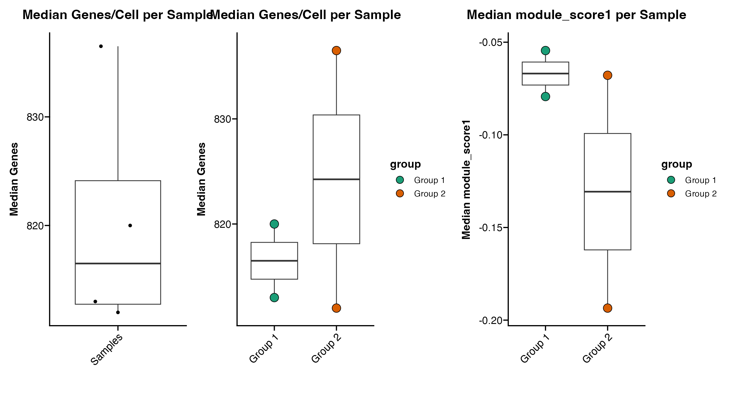
Plotting Median Data
scCustomize also contains series of functions for plotting the results of these median calculations:
Plot_Median_Genes(seurat_object = pbmc)

Plot_Median_Genes(seurat_object = pbmc, group.by = "group")

Plot_Median_Other(seurat_object = pbmc, median_var = "module_score1", group.by = "group")