Plotting #2: QC Plots & Analysis
Compiled: May 11, 2026
Source:vignettes/articles/QC_Plots.Rmd
QC_Plots.RmdQC Metrics & Plots
One of the first steps in all scRNA-seq analyses is performing a number of QC checks and plots so that data can be appropriately filtered. scCustomize contains a number of functions that can be used to quickly and easily generate some of the most relevant QC plots.
For details on functions for adding QC metrics and details about them please see Object QC Vignette.
For this tutorial, I will be utilizing HCA bone marrow cell data from the SeuratData package.
library(ggplot2)
library(dplyr)
library(magrittr)
library(patchwork)
library(Seurat)
library(scCustomize)
library(qs2)

# Load Example Dataset
hca_bm <- hcabm40k.SeuratData::hcabm40k

# Add pseudo group variable just for this vignette
hca_bm@meta.data$group[hca_bm@meta.data$orig.ident == "MantonBM1" | hca_bm@meta.data$orig.ident ==
    "MantonBM2" | hca_bm@meta.data$orig.ident == "MantonBM3" | hca_bm@meta.data$orig.ident == "MantonBM4"] <- "Group 1"

hca_bm@meta.data$group[hca_bm@meta.data$orig.ident == "MantonBM5" | hca_bm@meta.data$orig.ident ==
    "MantonBM6" | hca_bm@meta.data$orig.ident == "MantonBM7" | hca_bm@meta.data$orig.ident == "MantonBM8"] <- "Group 2"
hca_bm <- Add_Cell_QC_Metrics(object = hca_bm, species = "human")Plotting QC Metrics
scCustomize has a number of quick QC plotting options for ease of
use.
NOTE: Most scCustomize plotting functions contain ...
parameter to allow user to supply any of the parameters for the original
Seurat function that is being used under the hood.
VlnPlot-Based QC Plots
scCustomize contains a number of shortcut/wrapper functions for QC
plotting, which are wrappers around
Seurat::VlnPlot()/VlnPlot_scCustom.
-
QC_Plots_Genes()Plots genes/features per cell/nucleus. -
QC_Plots_UMIs()Plots UMIs per cell/nucleus.
-
QC_Plots_Mito()Plots mito% (named “percent_mito”) per cell/nucleus. -
QC_Plots_Complexity()Plots cell complexity metric (log10GenesPerUMI) per cell/nucleus. -
QC_Plots_Feature()Plots “feature” per cell/nucleus. Using parameterfeatureto allow plotting of any applicable named feature in object@meta.data slot. -
QC_Plots_Combined_Vln()Returns patchwork plot ofQC_Plots_Genes(),QC_Plots_UMIs(), &QC_Plots_Mito().
scCustomize functions have the added benefit of:
- Feature to plot set by default (except for
QC_Plots_Feature). - Added high/low cutoff parameters to allow for easy visualization of potential cutoff thresholds.
# All functions contain
p1 <- QC_Plots_Genes(seurat_object = hca_bm, low_cutoff = 600, high_cutoff = 5500)
p2 <- QC_Plots_UMIs(seurat_object = hca_bm, low_cutoff = 1200, high_cutoff = 45000)
p3 <- QC_Plots_Mito(seurat_object = hca_bm, high_cutoff = 20)
p4 <- QC_Plots_Complexity(seurat_object = hca_bm, high_cutoff = 0.8)
wrap_plots(p1, p2, p3, p4, ncol = 4)
Additional parameters
In addition to being able to supply Seurat parameters with
... these plots like many others in scCustomize contain
other additional parameters to customize plot output without need for
post-plot ggplot2 modifications
-
plot_title: Change plot title -
x_axis_label/y_axis_label: Change axis labels. -
x_lab_rotate: Should x-axis label be rotated 45 degrees? -
y_axis_log: Should y-axis in linear or log10 scale.
-
plot_median&median_size: Plot a line at the median of each x-axis identity.
-
plot_boxplot: Plot boxplot on top of the violin.
p1 <- QC_Plots_UMIs(seurat_object = hca_bm, low_cutoff = 1200, high_cutoff = 45000, pt.size = 0.1)
p2 <- QC_Plots_UMIs(seurat_object = hca_bm, low_cutoff = 1200, high_cutoff = 45000, pt.size = 0.1,
    y_axis_log = TRUE)

wrap_plots(p1, p2, ncol = 2)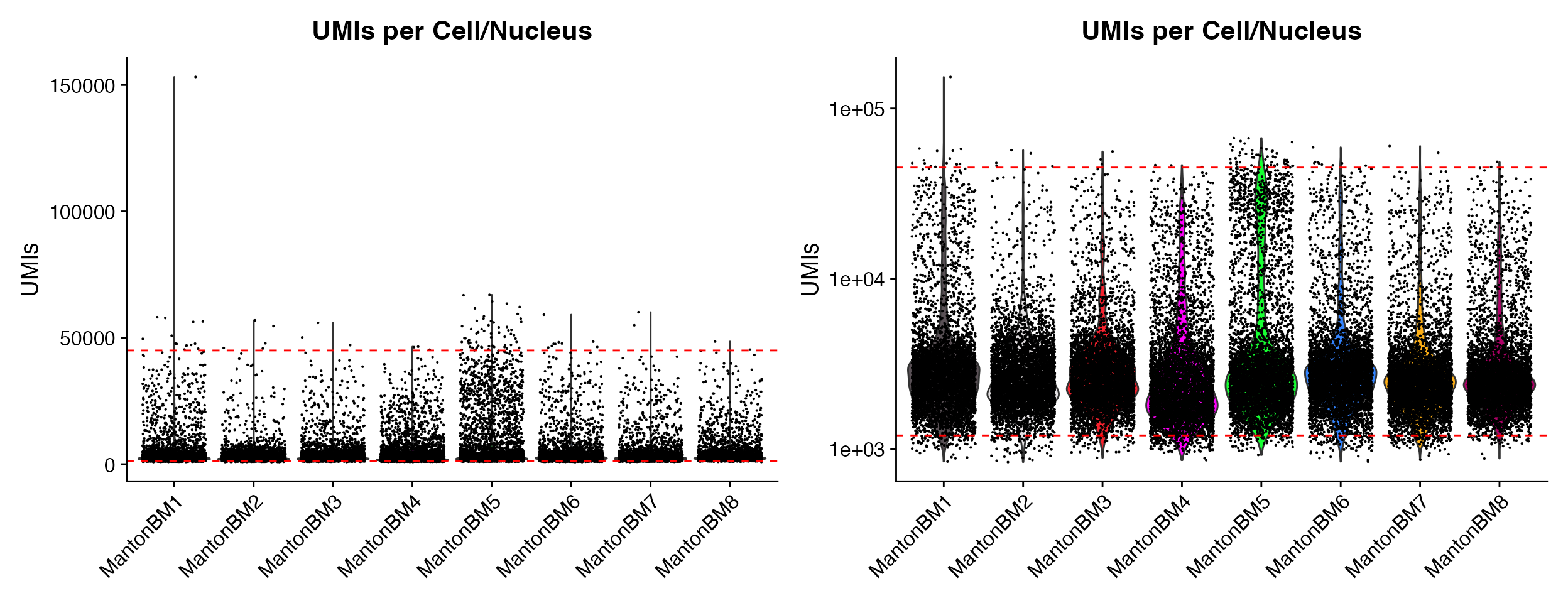
Setting y_axis_log can be very helpful for initial
plots where outliers skew the visualization of the majority of the data
without excluding data by setting y-axis limit.
p1 <- QC_Plots_UMIs(seurat_object = hca_bm, low_cutoff = 1200, high_cutoff = 45000, pt.size = 0,
    plot_median = TRUE)
p2 <- QC_Plots_UMIs(seurat_object = hca_bm, low_cutoff = 1200, high_cutoff = 45000, pt.size = 0,
    y_axis_log = TRUE, plot_median = TRUE)

wrap_plots(p1, p2, ncol = 2)
Plotting median values by setting the
plot_median = TRUE parameter.
p1 <- QC_Plots_UMIs(seurat_object = hca_bm, low_cutoff = 1200, high_cutoff = 45000, pt.size = 0,
    plot_boxplot = TRUE)
p2 <- QC_Plots_UMIs(seurat_object = hca_bm, low_cutoff = 1200, high_cutoff = 45000, pt.size = 0,
    y_axis_log = TRUE, plot_boxplot = TRUE)

wrap_plots(p1, p2, ncol = 2)
Plotting boxplot by setting the plot_boxplot = TRUE
parameter.
Combined Plotting Function
As a shortcut you can return single patchwork plot of the 3 main QC
Plots (Genes, UMIs, %Mito) by using single function,
QC_Plots_Combined_Vln().
QC_Plots_Combined_Vln(seurat_object = hca_bm, feature_cutoffs = c(600, 5500), UMI_cutoffs = c(1200,
    45000), mito_cutoffs = 20, pt.size = 0.1)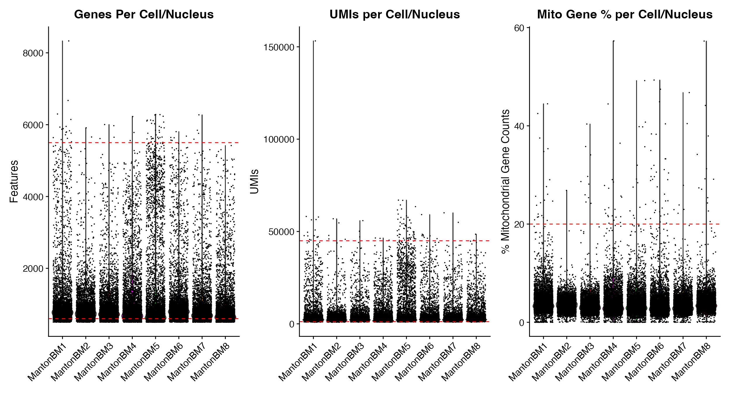
FeatureScatter-Based QC Plots
scCustomize contains 3 functions which wrap
Seurat::FeatureScatter() with added visualization of
potential cutoff thresholds and some additional functionality:
-
QC_Plot_UMIvsGene()Plots genes vs UMIs per cell/nucleus -
QC_Plot_GenevsFeature()Plots Genes vs. “feature” per cell/nucleus. Using parameterfeature1to allow plotting of any applicable named feature in object@meta.data slot.
-
QC_Plot_UMIvsFeature()Plots UMIs vs. “feature” per cell/nucleus. Using parameterfeature1to allow plotting of any applicable named feature in object@meta.data slot.
New/Modified functionality
- Better default color palettes
-
shuffle = TRUEby default to prevent hiding of datasets - Ability to set & visualize potential cutoff thresholds (similar to VlnPlot based QC Plots above)
- Report potential post filtering correlation in addition to whole
dataset correlation when using
QC_Plot_UMIvsGene(based on values provided to high and low cutoff parameters)
# All functions contain
QC_Plot_UMIvsGene(seurat_object = hca_bm, low_cutoff_gene = 600, high_cutoff_gene = 5500, low_cutoff_UMI = 500,
    high_cutoff_UMI = 50000)
QC_Plot_GenevsFeature(seurat_object = hca_bm, feature1 = "percent_mito", low_cutoff_gene = 600,
    high_cutoff_gene = 5500, high_cutoff_feature = 20)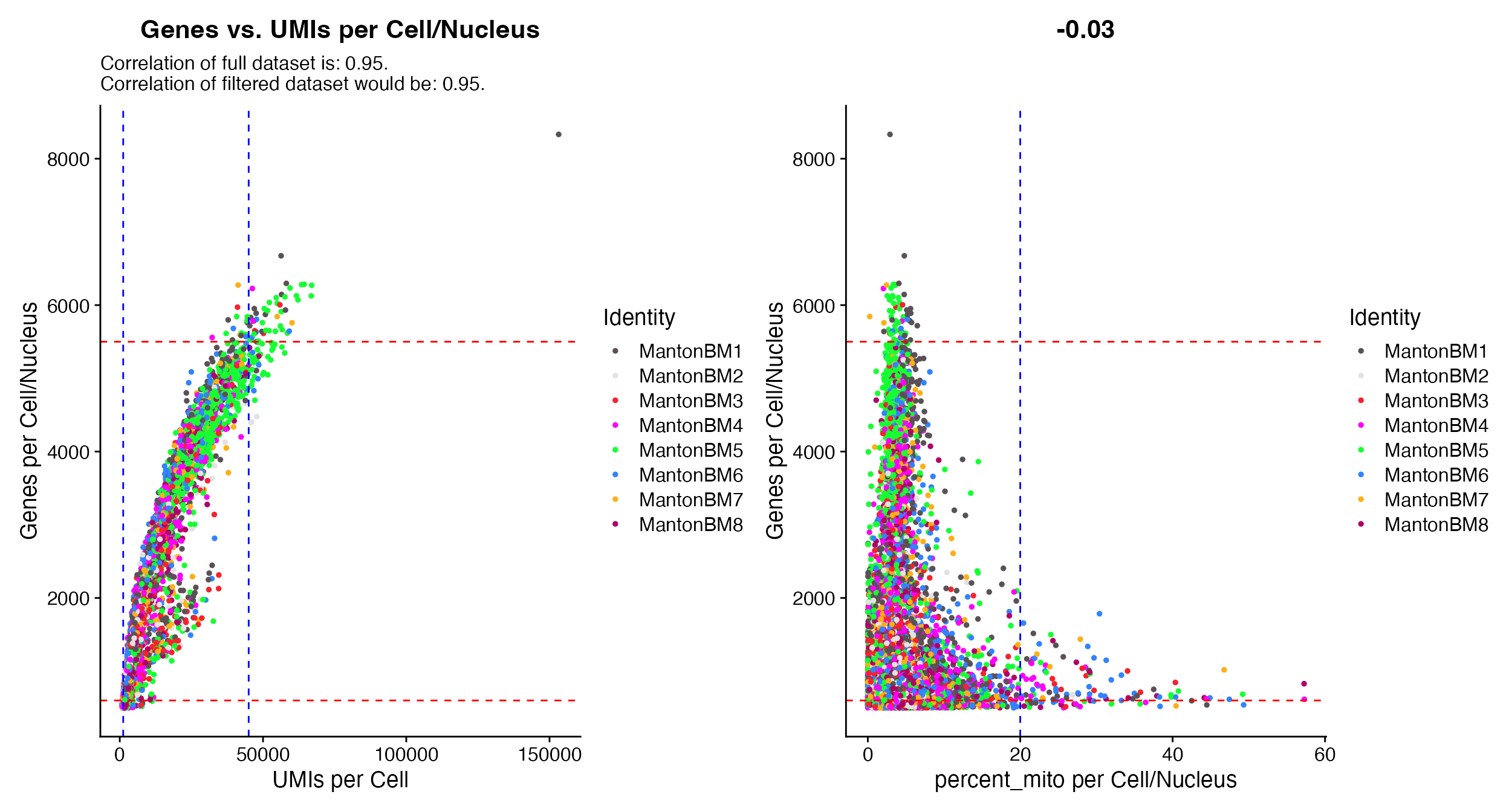
Color data by continuous meta data variable
QC_Plot_UMIvsGene contains the ability to color points
by continuous meta data variables.
This can be used to plot % of mito reads in addition to UMI vs. Gene
comparisons
QC_Plot_UMIvsGene(seurat_object = hca_bm, meta_gradient_name = "percent_mito", low_cutoff_gene = 600,
    high_cutoff_gene = 5500, high_cutoff_UMI = 45000)
QC_Plot_UMIvsGene(seurat_object = hca_bm, meta_gradient_name = "percent_mito", low_cutoff_gene = 600,
    high_cutoff_gene = 5500, high_cutoff_UMI = 45000, meta_gradient_low_cutoff = 20)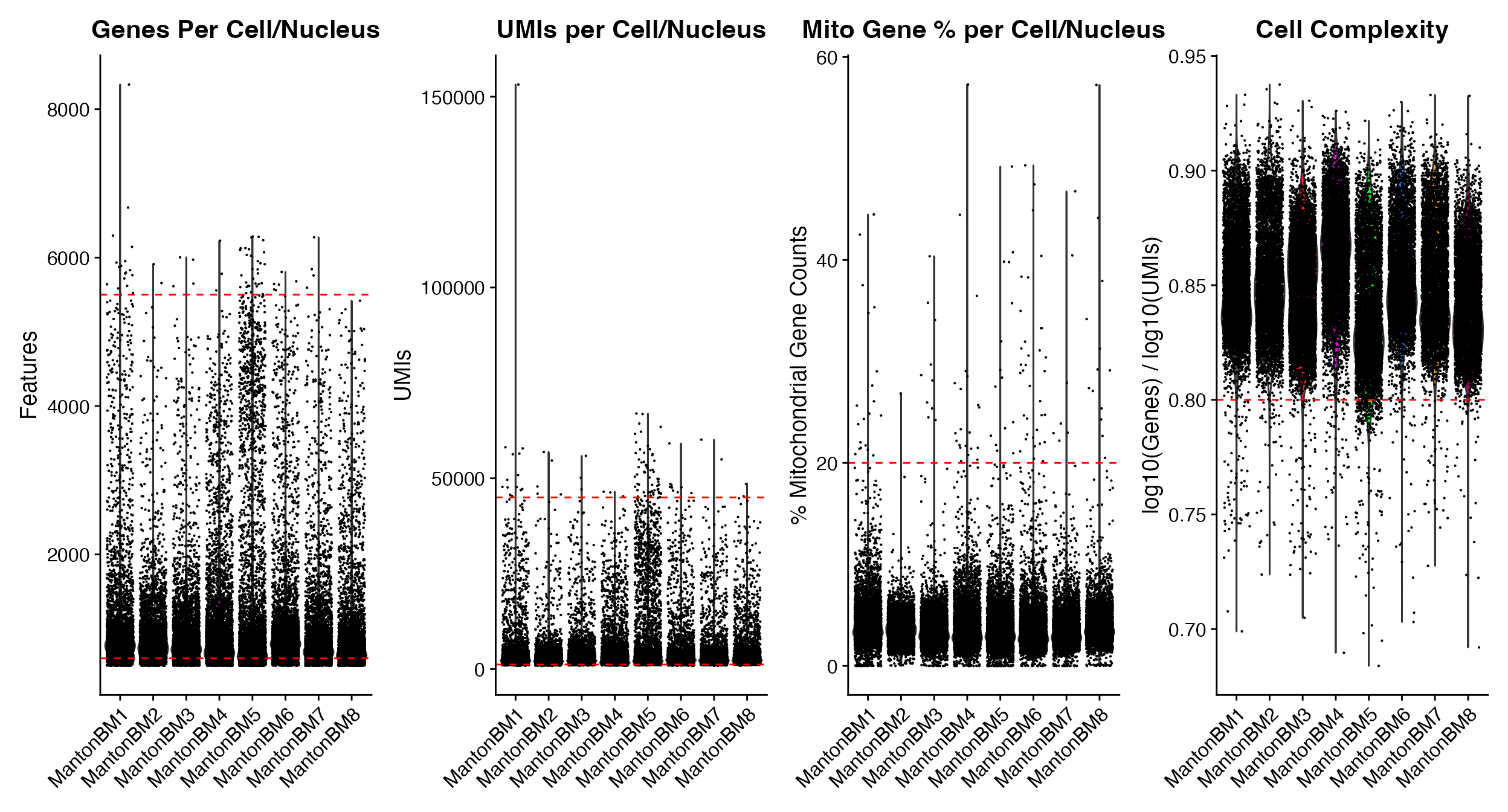
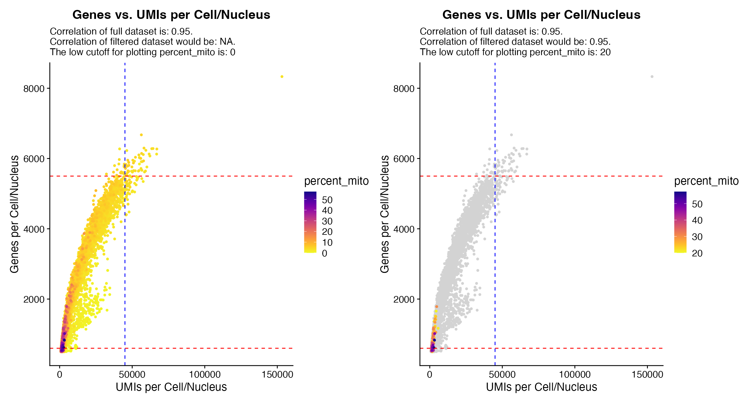
QC_Plot_UMIvsGene() when using
meta_gradient_name outputs plot colored by meta data
variable (left) to view only points above potential cutoff
meta_gradient_low_cutoff can be specified to alter the
plotting (right).
Combination Plots
If you are interested in viewing QC_Plot_UMIvsGene both
by discrete grouping variable and by continuous variable without writing
function twice you can use combination = TRUE and plot
output will contain both plots.
QC_Plot_UMIvsGene(seurat_object = hca_bm, meta_gradient_name = "percent_mito", low_cutoff_gene = 600,
    high_cutoff_gene = 5500, high_cutoff_UMI = 45000, meta_gradient_low_cutoff = 20, combination = TRUE)
QC_Plot_UMIvsGene() when using
combination = TRUE will output both the Gene x UMI by
active identity and with meta data gradient coloring.
Histogram-Based QC Plots
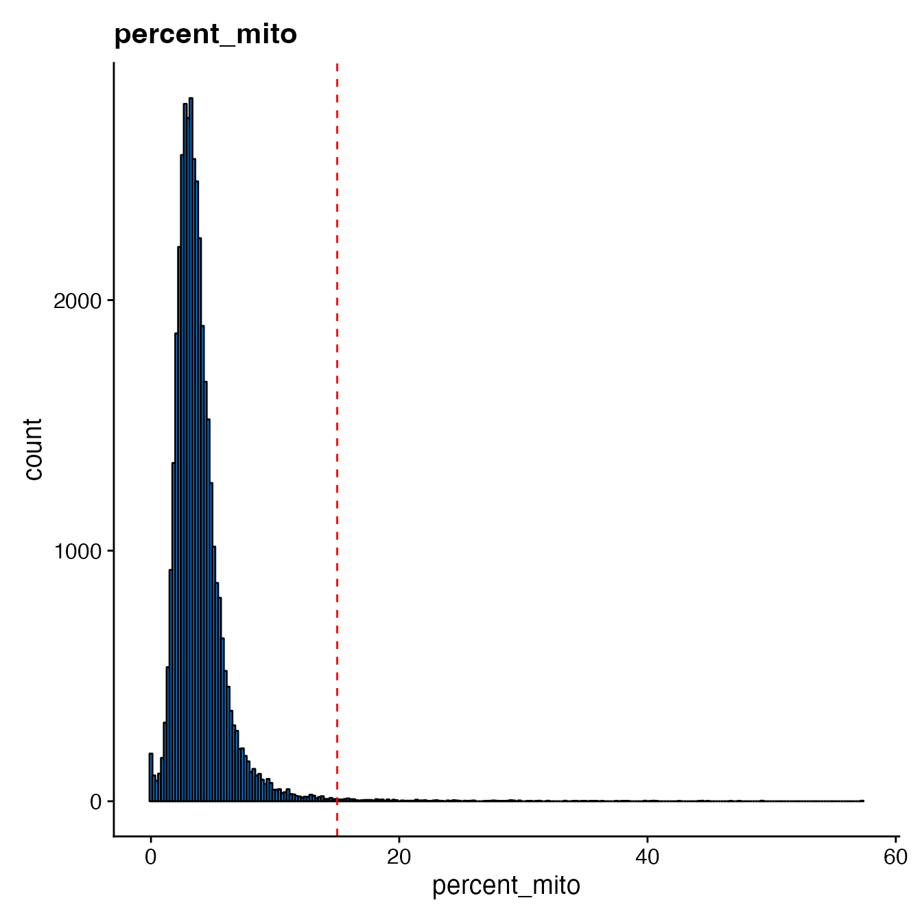
Finally, scCustomize contains a function to plot QC metrics as histogram instead of violin for visualization of the distribution of feature.
QC_Histogram(seurat_object = hca_bm, features = "percent_mito", low_cutoff = 15)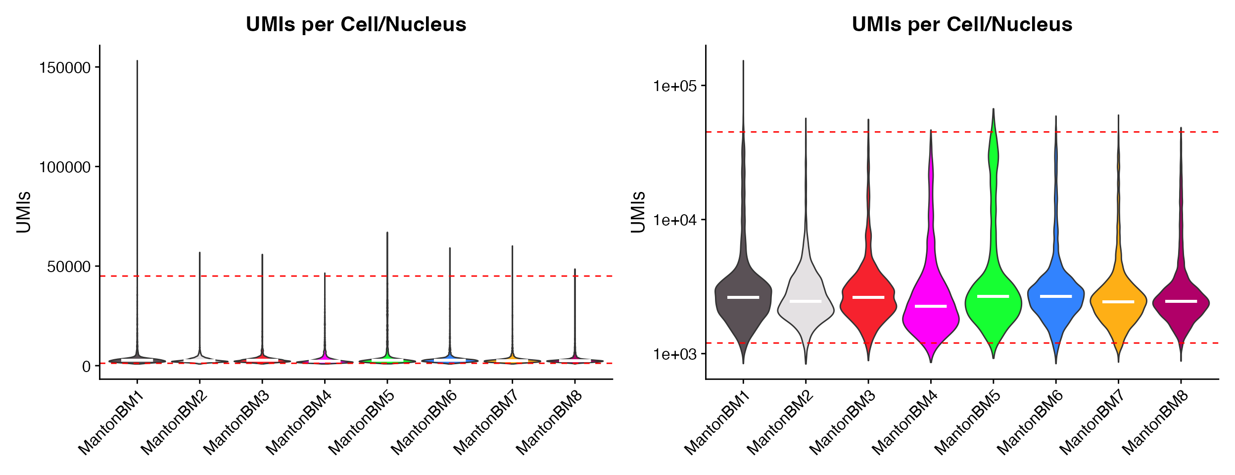
QC_Histogram(seurat_object = hca_bm, features = "percent_mito", low_cutoff = 15, split.by = "group")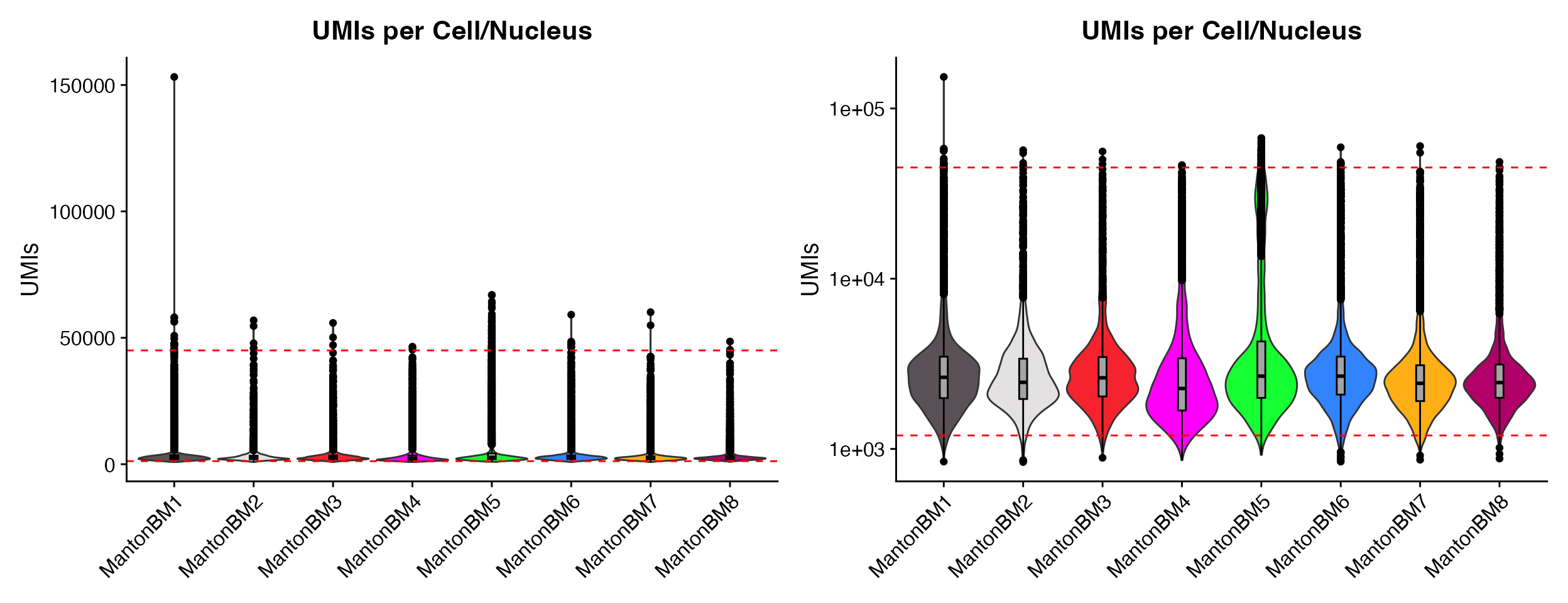
QC_Histogram also supports splitting plots by meta.data
variables
Analyze Median QC Values per Sample/Library
scCustomize also contains a few helpful functions for returning and plotting the median values for these metrics on per sample/library basis.
Calculate Median Values & Return data.frame
scCustomize contains function Median_Stats to quickly
calculate the medians for basic QC stats (Genes/, UMIs/, %Mito/Cell,
etc) and return a data.frame.
median_stats <- Median_Stats(seurat_object = hca_bm, group.by = "orig.ident")| orig.ident | Median_nCount_RNA | Median_nFeature_RNA | Median_percent_mito | Median_percent_ribo | Median_percent_mito_ribo | Median_log10GenesPerUMI |
|---|---|---|---|---|---|---|
| MantonBM1 | 2634.5 | 807 | 3.928074 | 42.04921 | 46.43790 | 0.8506316 |
| MantonBM2 | 2462.5 | 783 | 3.556994 | 42.96184 | 46.87269 | 0.8505270 |
| MantonBM3 | 2617.0 | 769 | 3.301410 | 40.65558 | 44.10722 | 0.8483425 |
| MantonBM4 | 2264.0 | 780 | 3.384891 | 33.73245 | 37.96850 | 0.8645139 |
| MantonBM5 | 2677.0 | 741 | 3.265677 | 41.55203 | 45.33713 | 0.8360196 |
| MantonBM6 | 2677.0 | 835 | 3.202053 | 43.07874 | 46.70119 | 0.8522162 |
| MantonBM7 | 2429.0 | 732 | 3.216184 | 44.68831 | 48.20765 | 0.8477172 |
| MantonBM8 | 2453.0 | 701 | 3.697331 | 44.97911 | 48.96420 | 0.8406128 |
| Totals (All Cells) | 2524.0 | 769 | 3.447040 | 41.53183 | 45.40989 | 0.8494067 |
The Median_Stats function has some column names stored
by default but will also calculate medians for additional meta.data
columns using the optional median_var parameter
median_stats <- Median_Stats(seurat_object = hca_bm, group.by = "orig.ident", median_var = "meta_data_column_name")Plotting Median Values
scCustomize also contains a few functions to plot some of these median value calculations, which can be used on their own without need to return data.frame first.
-
Plot_Median_Genes()
-
Plot_Median_UMIs()
-
Plot_Median_Mito()
-
Plot_Median_Other()- Used to plot any other numeric variable present in object meta.data slot.
Plot_Median_Genes(seurat_object = hca_bm, group.by = "group")
Plot_Median_UMIs(seurat_object = hca_bm, group.by = "group")
Plot_Median_Mito(seurat_object = hca_bm, group.by = "group")
Plot_Median_Other(seurat_object = hca_bm, median_var = "percent_ribo", group.by = "group")