cNMF_Functionality & Plotting

Interaction with consensus non-negative matrix factorization (cNMF)

scCustomize contains functions to aid in the interaction with results of consensus non-negative matrix factorization (cNMF) and Seurat objects. For more information on cNMF see cNMF GitHub Repo and cNMF Publication.

For this example we will use example outputs from using the pbmc3k object run using the same paramters as shown in cNMF R vignette.

library(ggplot2)
library(dplyr)
library(tibble)
library(magrittr)
library(Seurat)
library(scCustomize)
library(patchwork)

# Load pbmc dataset
pbmc <- pbmc3k.SeuratData::pbmc3k

# Run basic analysis (copied from pbmc3k vignette)
pbmc <- NormalizeData(pbmc) %>%
    FindVariableFeatures() %>%
    ScaleData() %>%
    RunPCA() %>%
    FindNeighbors(dims = 1:10) %>%
    FindClusters(resolution = 0.5) %>%
    RunUMAP(dims = 1:10)

## Modularity Optimizer version 1.3.0 by Ludo Waltman and Nees Jan van Eck
## 
## Number of nodes: 2700
## Number of edges: 97892
## 
## Running Louvain algorithm...
## Maximum modularity in 10 random starts: 0.8719
## Number of communities: 9
## Elapsed time: 0 seconds

new.cluster.ids <- c("Naive CD4 T", "CD14+ Mono", "Memory CD4 T", "B", "CD8 T", "FCGR3A+ Mono",
    "NK", "DC", "Platelet")
names(new.cluster.ids) <- levels(pbmc)
pbmc <- RenameIdents(pbmc, new.cluster.ids)
DimPlot_scCustom(pbmc, label = TRUE, pt.size = 0.5) + NoLegend()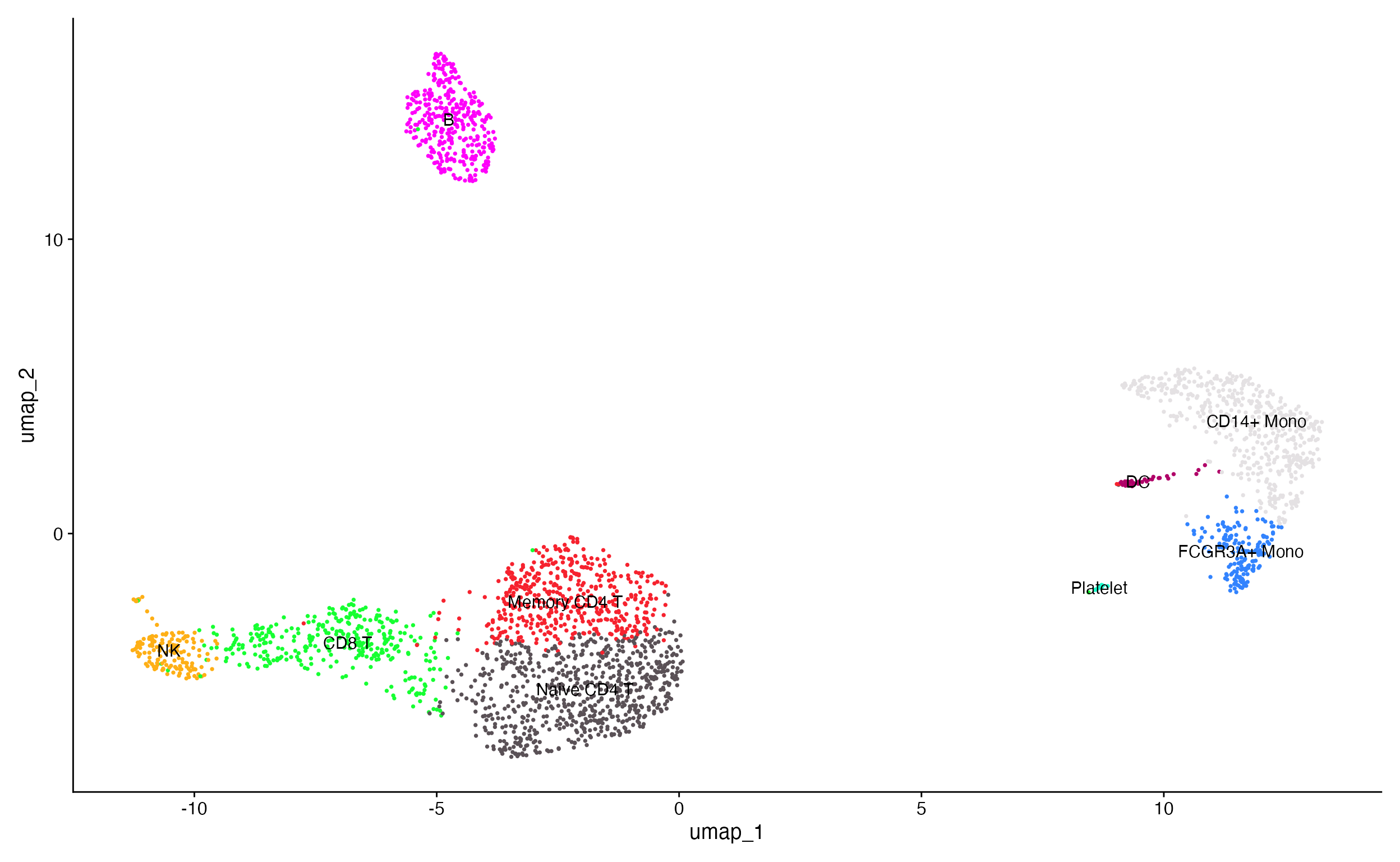

Loading the results of cNMF

scCustomize contains the function Read_Add_cNMF that can take the results from cNMF and add custom dimensionality reduction to Seurat object. The function only requires user to supply the paths to the cNMF usage and spectra files that contain the cell and feature loadings respectively. By default this will add new reduction “cnmf” to the Seurat object.

pbmc <- Read_Add_cNMF(seurat_object = pbmc, usage_file = "assets/cNMF_Example_Data/example_cNMF.usages.k_7.dt_0_1.consensus.txt",
    spectra_file = "assets/cNMF_Example_Data/example_cNMF.gene_spectra_score.k_7.dt_0_1.txt")

Optional parameters

There are few optional parameters in Read_Add_cNMF for increased user control if desired.
* reduction_name & reduction_key These can used to either change defaults (“cnmf” and “cNMF_” respectively) or if user wants to add results from multiple cNMF runs different names can be supplied for each one.
- For instance save second reduction with different k value.
* overwrite used to overwrite old cNMF reduction with new data using the same reduction_name.

# Add result from additional cNMF run as separate reduction (for instance with different k
# value)
pbmc <- Read_Add_cNMF(seurat_object = pbmc, usage_file = "assets/cNMF_Example_Data/example_cNMF.usages.k_15.dt_0_1.consensus.txt",
    spectra_file = "assets/cNMF_Example_Data/example_cNMF.gene_spectra_score.k_15.dt_0_1.txt", reduction_name = "cnmf.alt",
    reduction_key = "CNMFALT_")

# Overwrite current cNMF reduction with new results but keep same `reduction_name`
pbmc <- Read_Add_cNMF(seurat_object = pbmc, usage_file = "assets/cNMF_Example_Data/example_cNMF.usages.k_15.dt_0_1.consensus.txt",
    spectra_file = "assets/cNMF_Example_Data/example_cNMF.gene_spectra_score.k_15.dt_0_1.txt", overwrite = TRUE)

cNMF Plotting

cNMF results can be plotted in several ways using scCustomize.

Plotting factor loading

The cNMF factor cell loadings can be plotted like any other reduction using FeaturePlot_scCustom. Just supply the name of the factor like any other reduction.

FeaturePlot_scCustom(seurat_object = pbmc, features = c("cNMF_1", "cNMF_2", "cNMF_3", "cNMF_4"))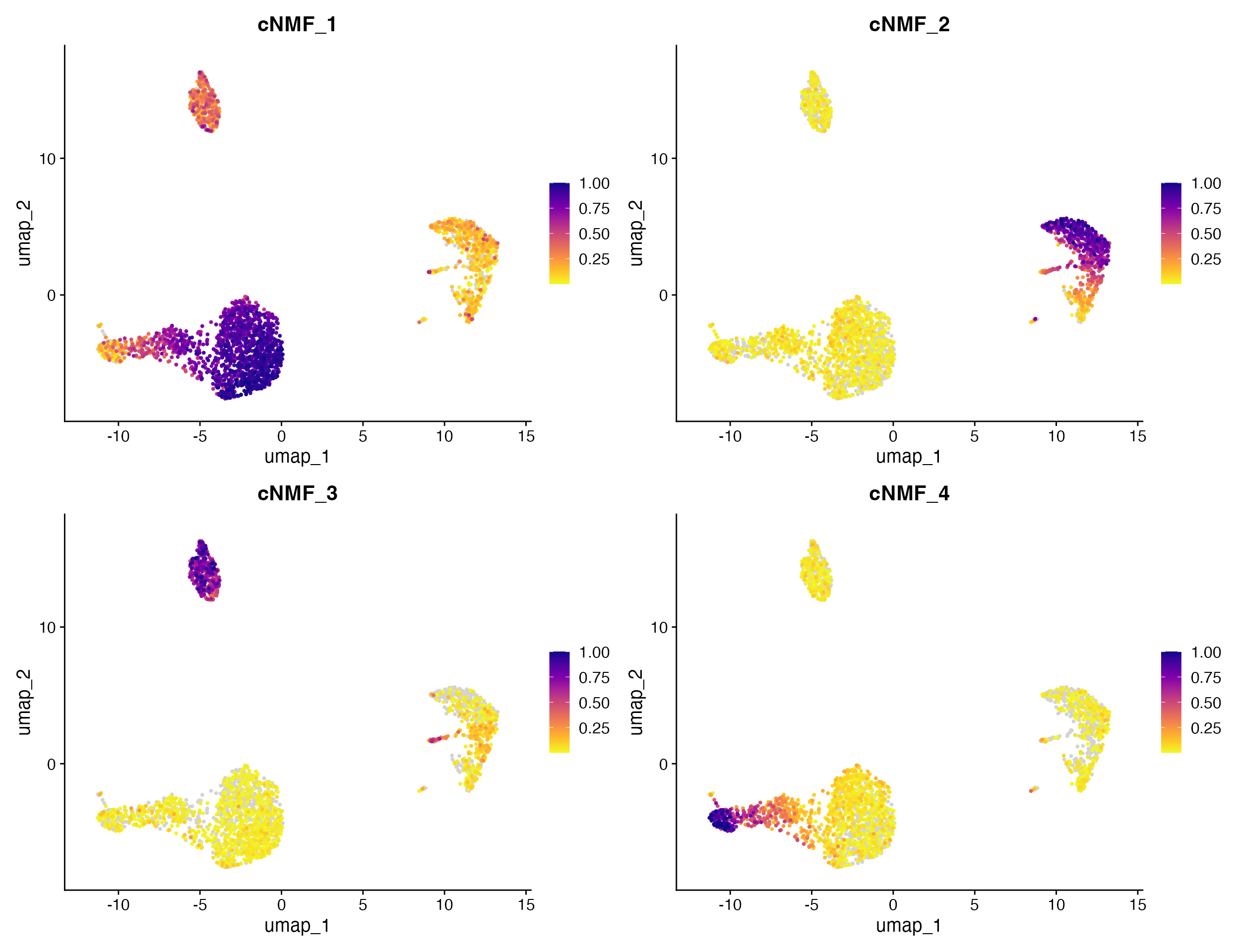

Plot factor correlation

scCustomize also has plotting function Factor_Cor_Plot to examine relationships between factors by plotting the correlation of feature loadings for cNMF factors.

Factor_Cor_Plot(object = pbmc, reduction = "cnmf")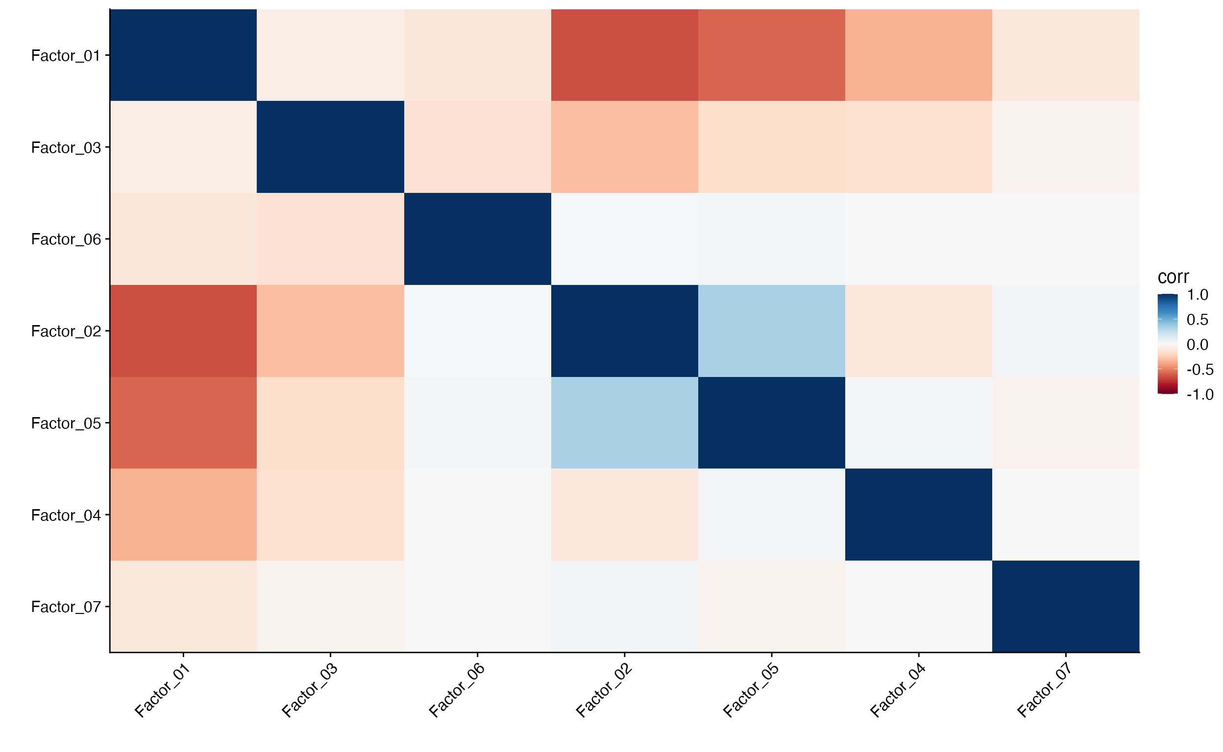

By default (above) Factor_Cor_Plot runs hierarchical clustering on the correlations and orders the factors on the plot. But users can also adjust this to plot the factors in numerical order.

Factor_Cor_Plot(object = pbmc, reduction = "cnmf", cluster = FALSE)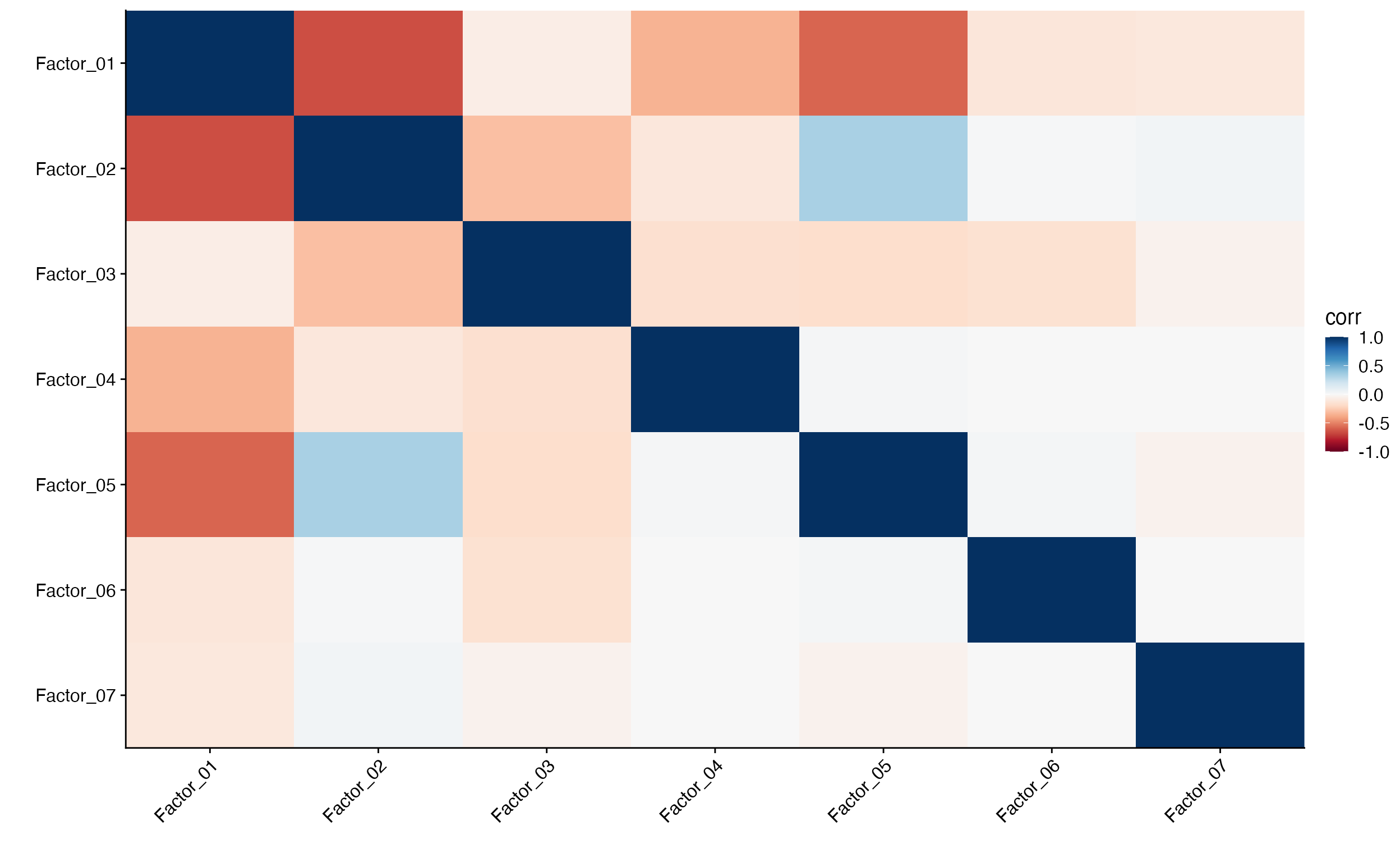

Factor_Cor_Plot also contains a number of other optional parameters to change the output plot.

# Only plot positive correlations
Factor_Cor_Plot(object = pbmc, reduction = "cnmf", positive_only = TRUE)

# Only plot only the upper diagonal
Factor_Cor_Plot(object = pbmc, reduction = "cnmf", plot_type = "upper", cluster = FALSE)

# Only plot only the lower diagonal
Factor_Cor_Plot(object = pbmc, reduction = "cnmf", plot_type = "lower", cluster = FALSE)

# Add clustering rectangles (uses `cutree`)
Factor_Cor_Plot(object = pbmc, reduction = "cnmf", cluster_rect = T, cluster_rect_num = 6, cluster_rect_col = "magenta")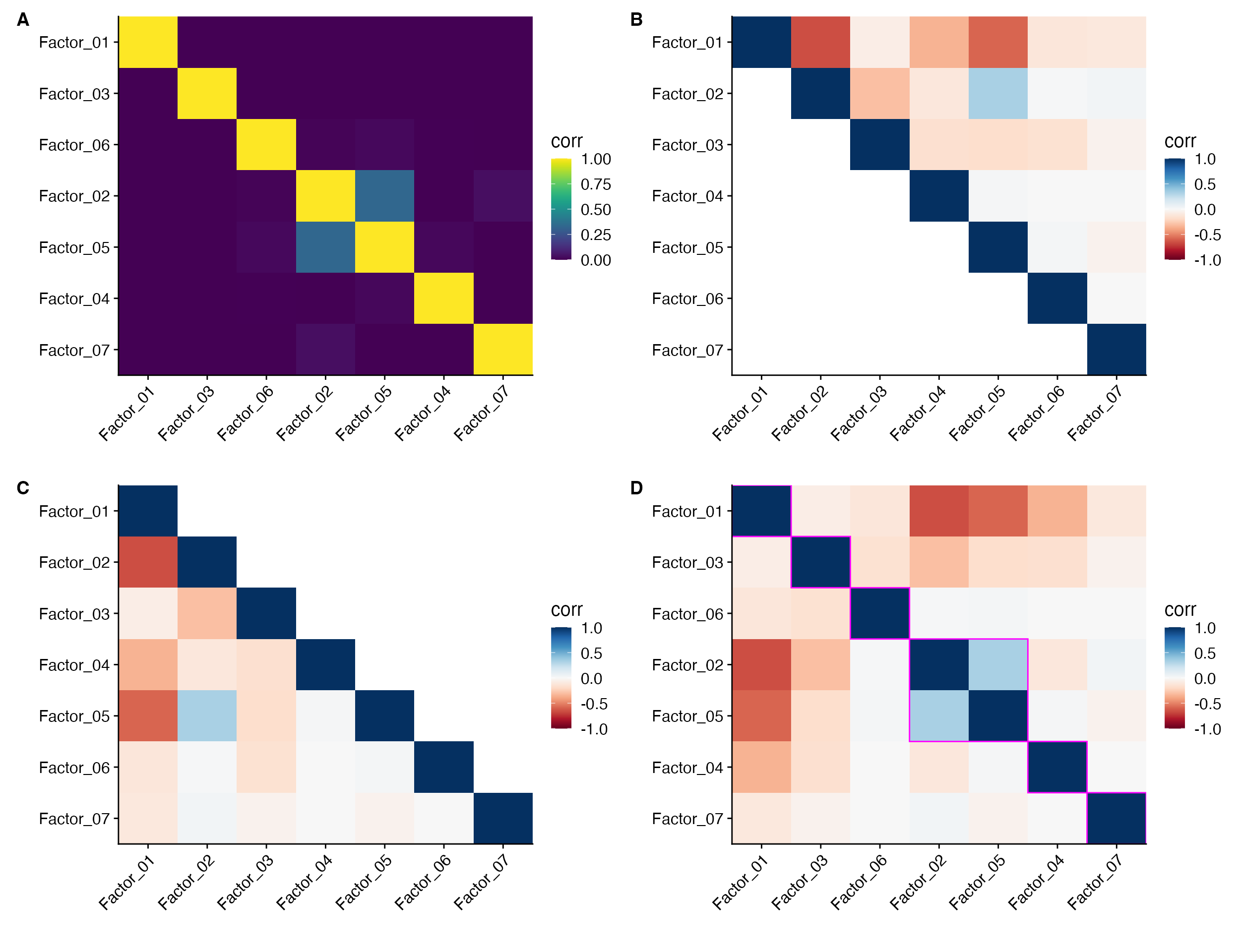

A. Plotting only the positive correlations (negative correlations set to 0). B. Plot only the upper diagonal (must set cluster = FALSE). C. Plot only the lower diagonal (must set cluster = FALSE). D. Add rectangles around clustered results (uses cutree).

cNMF Interaction

scCustomize also contains functions to interact with and retrive data from the cNMF reduction.
NOTE: These functions are S3 generics and can be used to retrieve the same information about LIGER iNMF reductions with given LIGER object, or from iNMF reduction in Seurat object.

The function Top_Genes_Factor can be used to retrieve top loading genes from cNMF factors. Let’s check what genes load most heavily on factor 2 which we can see above loads heavily on CD14+ Monocyte cluster.

top_gene_factor1 <- Top_Genes_Factor(object = pbmc, factor = 2, reduction = "cnmf")

top_gene_factor1

##  [1] "LGALS1" "GSTP1"  "LGALS2" "TYROBP" "FCN1"   "CST3"   "CD14"   "S100A8"
##  [9] "S100A9" "LYZ"

By default Top_Genes_Factor will return the top 10 loading genes but can return any number of genes by supplying value to the num_genes parameter.

top_gene_factor1 <- Top_Genes_Factor(object = pbmc, factor = 2, num_genes = 20, reduction = "cnmf")

top_gene_factor1

##  [1] "CSF3R"   "GABARAP" "TYMP"    "BLVRB"   "FTL"     "GRN"     "TSPO"   
##  [8] "CEBPD"   "S100A6"  "AP1S2"   "LGALS1"  "GSTP1"   "LGALS2"  "TYROBP" 
## [15] "FCN1"    "CST3"    "CD14"    "S100A8"  "S100A9"  "LYZ"

If you want to retrieve the top loading genes for all factors within given reduction you can set factor = "all" and the function will return data.frame with one column per factor.

top_10_factor_df <- Top_Genes_Factor(object = pbmc, factor = "all", reduction = "cnmf")

head(top_10_factor_df, 10)

	Factor_1	Factor_2	Factor_3	Factor_4	Factor_5	Factor_6	Factor_7
1	HLA-DRB1	LGALS1	HLA-DPA1	CLIC3	AIF1	BLM	PRUNE
2	CYBA	GSTP1	MS4A1	CTSW	RHOC	BIRC5	ESAM
3	RPS27A	LGALS2	HLA-DQA2	CST7	COTL1	KIFC1	MMD
4	RPS6	TYROBP	CD79B	SPON2	IFITM2	TK1	PTCRA
5	RPL31	FCN1	HLA-DRB1	FGFBP2	IFITM3	CDC20	ACRBP
6	RPS15A	CST3	HLA-DPB1	GNLY	MS4A7	KIAA0101	LGALSL
7	EEF1A1	CD14	HLA-DQA1	GZMA	RP11-290F20.3	TYMS	AC147651.3
8	RPS25	S100A8	HLA-DQB1	GZMB	LST1	MCM10	HIST1H2AC
9	RPS27	S100A9	HLA-DRA	PRF1	FCER1G	CDC6	TSC22D1
10	RPS12	LYZ	CD74	NKG7	FCGR3A	RRM2	C2orf88